Introduction to Number Fields¶

In Sage, we can create the number field $\mathbb{Q}(\sqrt[3]{2})$ as follows.

sage: K.<alpha> = NumberField(x^3 - 2)

The above creates two Sage objects, $K$ and $\alpha$ . Here $K$ “is” (isomorphic to) the number field $\mathbb{Q}(\sqrt[3]{2})$ , as we confirm below:

sage: K
Number Field in alpha with defining polynomial x^3 - 2

and $\alpha$ is a root of $x^3 - 2$ , so $\alpha$ is an abstract choice of $\sqrt[3]{2}$ (no specific embedding of the number field $K$ into $\mathbb{C}$ is chosen by default in Sage-3.1.2):

sage: alpha^3
2
sage: (alpha+1)^3
3*alpha^2 + 3*alpha + 3

The variable $x$ ¶

Note that we did not define $x$ above before using it. You could “break” the above example by redefining $x$ to be something funny:

sage: x = 1
sage: K.<alpha> = NumberField(x^3 - 2)
...
TypeError: polynomial (=-1) must be a polynomial.

The Traceback above indicates that there was an error. Potentially lots of detailed information about the error (a “traceback”) may be given after the word Traceback and before the last line, which contains the actual error messages.

Note

Important: whenever you use Sage and get a big error, look at the last line for the actual error, and only look at the rest if you are feeling adventurous. In the notebook, the part indicated by ... above is not displayed; to see it, click just to the left of the word Traceback and the traceback will appear.

If you redefine $x$ as above, but need to define a number field using the indeterminate $x$ , you have several options. You can reset $x$ to its default value at the start of Sage, you can redefine $x$ to be a symbolic variable, or you can define $x$ to be a polynomial indeterminant (a polygen):

sage: reset('x')
sage: x
x
sage: x = 1
sage: x = var('x')
sage: x
x
sage: x = 1
sage: x = polygen(QQ, 'x')
sage: x
x
sage: x = 1
sage: R.<x> = PolynomialRing(QQ)
sage: x
x

Using tab completion to get the methods of an object¶

One you have created a number field $K$ , type K.[tab key] to see a list of functions. Type, e.g., K.Minkowski_embedding?[tab key] to see help on the Minkowski_embedding command. To see source code, type K.Minkowski_embedding??[tab key].

sage: K.<alpha> = NumberField(x^3 - 2)
sage: K.[tab key]

Symbolic Expressions¶

Another natural way for us to create certain number fields is to create a symbolic expression and adjoin it to the rational numbers. Unlike Pari and Magma (and like Mathematica and Maple), Sage also supports manipulation of symbolic expressions and solving equations, without defining abstract structures such as a number fields. For example, we can define a variable $a=\sqrt{2}$ as an abstract symbolic object by simply typing a = sqrt(2). When we type parent(a) below, Sage tells us the mathematical object that it views $a$ as being an element of; in this case, it’s the ring of all symbolic expressions.

sage: a = sqrt(2)
sage: parent(a)
Symbolic Ring

sqrt(2) in Pari and Magma¶

In particular, typing sqrt(2) does not numerically extract an approximation to $\sqrt{2}$ , like it would in Pari or Magma. We illustrate this below by calling Pari (via the gp interpreter) and Magma directly from within Sage. After we evaluate the following two input lines, copies of GP/Pari and Magma are running, and there is a persistent connection between Sage and those sessions.

sage: gp('sqrt(2)')
1.414213562373095048801688724
sage: magma('Sqrt(2)')                  # optional
1.41421356237309504880168872421

You probably noticed a pause when evaluated the second line as Magma started up. Also, note the # optional comment, which indicates that the line won’t work if you don’t have Magma installed.

Numerically evaluating sqrt(2)¶

Incidentally, if you want to numerically evaluate $\sqrt{2}$ in Sage, just give the optional prec argument to the sqrt function, which takes the required number of bits (binary digits) of precision.

sage: sqrt(2, prec=100)
1.4142135623730950488016887242

It’s important to note in computations like this that there is not an a priori guarantee that prec bits of the answer are all correct. Instead, what happens is that Sage creates the number $2$ as a floating point number with $100$ bits of accuracy, then asks Paul Zimmerman’s MPFR C library to compute the square root of that approximate number.

Arithmetic with sqrt(2)¶

We return now to our symbolic expression $a = \sqrt{2}$ . If you ask to square $a+1$ you simply get the formal square. To expand out this formal square, we use the expand command.

sage: a = sqrt(2)
sage: (a+1)^2
(sqrt(2) + 1)^2
sage: expand((a+1)^2)
2*sqrt(2) + 3

Adjoining a symbolic expression¶

Given any symbolic expression for which Sage can computes its minimal polynomial, you can construct the number field obtained by adjoining that expression to $\mathbb{Q}$ . The notation is quite simple - just type QQ[a] where a is the symbolic expression.

sage: a = sqrt(2)
sage: K.<b> = QQ[a]
sage: K
Number Field in sqrt2 with defining polynomial x^2 - 2
sage: b
sqrt2
sage: (b+1)^2
2*sqrt2 + 3
sage: QQ[a/3 + 5]
Number Field in a with defining polynomial x^2 - 10*x + 223/9

Coercion: QQ[a] versus QQ(a)¶

You can’t create the number field $\mathbb{Q}(a)$ in Sage by typing QQ(a), which has a very different meaning in Sage. It means “try to create a rational number from $a$ .” Thus QQ(a) in Sage is the analogue of QQ!a in Magma (Pari has no notion of rings such as QQ).

sage: a = sqrt(2)
sage: QQ(a)
...
TypeError: unable to convert sqrt(2) to a rational

In general, if $X$ is a ring, or vector space or other “parent structure” in Sage, and $a$ is an element, type X(a) to make an element of $X$ from $a$ . For example, if $X$ is the finite field of order $7$ , and $a=2/5$ is a rational number, then X(a) is the finite field element $6$ (as a quick exercise, check that this is mathematically the correct interpretation).

sage: X = GF(7); a = 2/5
sage: X(a)
6

Solving a cubic equation¶

As a slightly less trivial illustration of symbolic manipulation, consider the cubic equation

$x^3 + \sqrt{2} x + 5 = 0.$

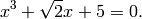
In Sage, we can create this equation, and find an exact symbolic solution.

sage: x = var('x')
sage: eqn =  x^3 + sqrt(2)*x + 5 == 0
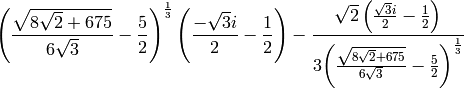
sage: a = solve(eqn, x)[0].rhs()

The first line above makes sure that the symbolic variable $x$ is defined, the second creates the equation eqn, and the third line solves eqn for $x$ , extracts the first solution (there are three), and takes the right hand side of that solution and assigns it to the variable a.

Viewing complicated symbolic expressions¶

To see the solution nicely typeset, use the show command:

sage: show(a)
{{\left(...

${{\left( \frac{\sqrt{ {8 \sqrt{ 2 }} + 675 }}{{6 \sqrt{ 3 }}} - \frac{5}{2} \right)}^{\frac{1}{3}} \left( \frac{{-\sqrt{ 3 } i}}{2} - \frac{1}{2} \right)} - \frac{{\sqrt{ 2 } \left( \frac{{\sqrt{ 3 } i}}{2} - \frac{1}{2} \right)}}{{3 {\left( \frac{\sqrt{ {8 \sqrt{ 2 }} + 675 }}{{6 \sqrt{ 3 }}} - \frac{5}{2} \right)}^{\frac{1}{3}} }}$

You can also see the latex needed to paste $a$ into a paper by typing latex(a). The latex command works on most Sage objects.

sage: latex(a)
{{\left( \frac{\sqrt{ {8 \sqrt{ 2 }} ...

Adjoining a root of the cubic¶

Next, we construct the number field obtained by adjoining the solution a to $\mathbb{Q}$ . Notice that the minimal polynomial of the root is $x^6 + 10x^3 - 2x^2 + 25$ .

sage: K.<b> = QQ[a]
sage: K
Number Field in a with defining
polynomial x^6 + 10*x^3 - 2*x^2 + 25
sage: a.minpoly()
x^6 + 10*x^3 - 2*x^2 + 25
sage: b.minpoly()
x^6 + 10*x^3 - 2*x^2 + 25

We can now compute interesting invariants of the number field $K$ :

sage: K.class_number()
5
sage: K.galois_group().order()
72

Introduction to Number Fields¶

The variable $x$ ¶

Using tab completion to get the methods of an object¶

Symbolic Expressions¶

sqrt(2) in Pari and Magma¶

Numerically evaluating sqrt(2)¶

Arithmetic with sqrt(2)¶

Adjoining a symbolic expression¶

Coercion: QQ[a] versus QQ(a)¶

Solving a cubic equation¶

Viewing complicated symbolic expressions¶

Adjoining a root of the cubic¶

Table Of Contents

Previous topic

Next topic

This Page

Quick search

Navigation

Introduction to Number Fields¶

The variable ¶

Using tab completion to get the methods of an object¶

Symbolic Expressions¶

sqrt(2) in Pari and Magma¶

Numerically evaluating sqrt(2)¶

Arithmetic with sqrt(2)¶

Adjoining a symbolic expression¶

Coercion: QQ[a] versus QQ(a)¶

Solving a cubic equation¶

Viewing complicated symbolic expressions¶

Adjoining a root of the cubic¶

Table Of Contents

Previous topic

Next topic

This Page

Quick search

Navigation

The variable $x$ ¶